Convolutional Neural Network MNIST Example Explained

We explain in detail Julia’s model-zoo example of a convolutional neural network, from a beginner’s perspective, so that we can understand the code well enough to modify it to work for another classification task.

Background

A student, Stephen Gibson, wanted to use a convolutional neural network to classify videos of skateboarding tricks. I want to learn Julia, so this seemed like a nice application to motivate me to learn something new. My strategy is to comment the existing code in great detail, along with what I don’t understand, so that we can adapt this code to our video classification task.

In other words, this is my first time looking at actual neural networks in code, or using software for neural networks, so I have no idea what I’m doing. Keep that in mind as you read. 😘

Julia’s model-zoo package has many examples of using Julia for machine learning. The code that follows comes from model-zoo’s example of applying a convolutional neural network to the MNIST data set. Download the whole script here. The MNIST data set is a set of images containing handwritten digits, for example:

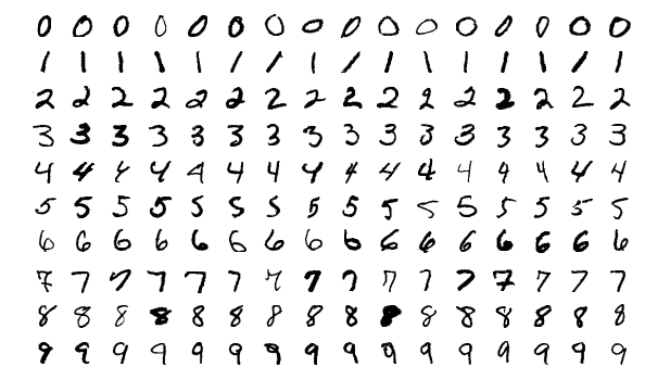
The goal of the program is to take these images and map them to the integers 0 through 9. Comments describe the high level goals of the program:

Demonstrates basic model construction, training, saving, conditional early-exit, and learning rate scheduling.

When you run it, the program prints the following output:

julia> using Pkg; Pkg.activate("."); Pkg.instantiate()
 Activating environment at `~/projects/SkateboardML/explorations/mnist/Project.toml`

julia> include("conv.jl")
[ Info: Loading data set
[ Info: Downloading MNIST dataset
...
[ Info: Building model...
[ Info: Beginning training loop...
[ Info: [1]: Test accuracy: 0.9739
[ Info:  -> New best accuracy! Saving model out to mnist_conv.bson
[ Info: [2]: Test accuracy: 0.9853
[ Info:  -> New best accuracy! Saving model out to mnist_conv.bson
...
[ Info: [15]: Test accuracy: 0.9810
┌ Warning:  -> Haven't improved in a while, dropping learning rate to 0.00030000000000000003!
└ @ Main ~/projects/SkateboardML/explorations/mnist/conv.jl:153
[ Info: [16]: Test accuracy: 0.9925
[ Info:  -> New best accuracy! Saving model out to mnist_conv.bson
...
[ Info: [20]: Test accuracy: 0.9929
[ Info:  -> New best accuracy! Saving model out to mnist_conv.bson
accuracy(test_set..., model) = 0.9929
0.9929

Watching the model improve at every iteration makes us a little more comfortable that it’s all working out as expected. Now we jump in and explain the code.

Imports

using Flux, Flux.Data.MNIST, Statistics
using Flux: onehotbatch, onecold, logitcrossentropy
using Base.Iterators: partition
using Printf, BSON
using Parameters: @with_kw
using CUDAapi

The code starts off by importing all the packages necessary for the task, very standard.

GPU

if has_cuda()
    @info "CUDA is on"
    import CuArrays
    CuArrays.allowscalar(false)
end

This block tests for CUDA GPU’s. Running a model on a GPU can make it much faster. The remainder of the code has calls to gpu() throughout, which presumably make that call run on the GPU.

My computer has two GPU’s, but they’re not nvidia, so I don’t have CUDA available. Happily, the code still worked just fine on my CPU. It would be nice if it worked out of the box on other GPU’s. The Julia GPU community seems quite active, and I suspect the infrastructure is available to run on other GPU’s with little modification to our application code.

On a syntactic note, @info is a macro for logging. Prefer these over print, because then you can adjust how verbose your program is without changing the code.

Global Parameters

@with_kw mutable struct Args
    lr::Float64 = 3e-3
    epochs::Int = 20
    batch_size = 128
    savepath::String = "./" 
end

The rest of the program passes Args around all over, so they act like global parameters. lr is the learning rate which controls They’re mutuable because the program dynamically adjusts them later based on how the training goes.

Transforming Images to Arrays

# Bundle images together with labels and group into minibatchess
function make_minibatch(X, Y, idxs)
    X_batch = Array{Float32}(undef, size(X[1])..., 1, length(idxs))
    for i in 1:length(idxs)
        X_batch[:, :, :, i] = Float32.(X[idxs[i]])
    end
    Y_batch = onehotbatch(Y[idxs], 0:9)
    return (X_batch, Y_batch)
end

This code transforms the grayscale images into Float32 arrays that Flux can process. A better name than make_minibatch might be transform_raw_inputs.

The definition of X_batch is Array{Float32}(undef, size(X[1])..., 1, length(idxs)). Here’s what each argument means:

• Array{Float32}(undef, the function call and the first argument, declares this as a Float32 array. There are no initial values, because we’ll fill them in later.
• size(X[1])...,, unpack into the two values, 28 and 28, which are the dimensions of the pixels in the image. This clever unpacking based on the value of x[1] means that the code will work with any set of images, as long as they’re all the same size. It should also unpack higher dimensions.
• 1, means the next (3rd) dimension has only 1 slice, because it’s a greyscale image. If the images were RGB color then this would be 3.
• length(idxs) says that the array will be as long as the number of images.

X_batch is a 4 dimensional Float32 array, with the last dimension corresponding to the sample, so X_batch[:, :, :, 1] is the first image. onehotbatch(Y[idxs], 0:9) encodes the labels Y[idxs] in a matrix of 1’s and 0’s, using 0:9 as the possible class values.

Loading Data

function get_processed_data(args)
    # Load labels and images from Flux.Data.MNIST
    train_labels = MNIST.labels()
    train_imgs = MNIST.images()
    mb_idxs = partition(1:length(train_imgs), args.batch_size)
    train_set = [make_minibatch(train_imgs, train_labels, i) for i in mb_idxs] 
    
    # Prepare test set as one giant minibatch:
    test_imgs = MNIST.images(:test)
    test_labels = MNIST.labels(:test)
    test_set = make_minibatch(test_imgs, test_labels, 1:length(test_imgs))

    return train_set, test_set

end

get_processed_data massages the data into the right form for the neural network. MNIST is a module that contains the actual MNIST data set. partition splits the images into groups so that each batch will have the same size.

Defining Model Architecture

# Build model
function build_model(args; imgsize = (28,28,1), nclasses = 10)
    cnn_output_size = Int.(floor.([imgsize[1]/8,imgsize[2]/8,32]))	

    return Chain(
    # First convolution, operating upon a 28x28 image
    Conv((3, 3), imgsize[3]=>16, pad=(1,1), relu),
    MaxPool((2,2)),

    # Second convolution, operating upon a 14x14 image
    Conv((3, 3), 16=>32, pad=(1,1), relu),
    MaxPool((2,2)),

    # Third convolution, operating upon a 7x7 image
    Conv((3, 3), 32=>32, pad=(1,1), relu),
    MaxPool((2,2)),

    # Reshape 3d tensor into a 2d one using `Flux.flatten`, at this point it should be (3, 3, 32, N)
    flatten,
    Dense(prod(cnn_output_size), 10))
end

build_model is a function that returns a function which actually defines the CNN. It returns a Chain representing the transformations in the network: three convolutions, each reducing the size of the dimensions, followed by a final densely connected layer. Google’s explanation of a convolution helped me understand the basic idea, and I recommend you look it over before proceeding.

Let’s examine Conv((3, 3), imgsize[3]=>16, pad=(1,1), relu) in detail. The first argument, (3, 3) defines the size of the convolution, so it operates on overlapping 3x3 pixels. It’s two dimensional, for a two dimensional image. If I’m going to write one that operates on a video, then it should be three dimensional. The second argument, imgsize[3]=>16, defines the input and output channels. imgsize[3] is just 1, so this convolution takes an input with 1 channel and produces an output with 16 channels. Coursera has an approachable video describing what it means to have multiple input and output channels. pad=(1,1) means that the sides of the input will be padded before the convolution, so the first two dimensions of the result will be the same size as the input. If we used a size (5, 5) convolution, then we would need pad=(2,2) to keep the first two dimensions the same. Finally, relu means the σ activation function is rectified linear unit. In summary, this convolution layer takes a 28 x 28 x 1 image and produces a 28 x 28 x 16 activation map.

The next function to apply is MaxPool((2,2)) for a max pooling layer to reduce the size of the output. (2,2) means that the max pooling will use 2 by 2 windows, which is common.

On a side note, I’m not sure why imgsize is hardcoded in as a default argument at (28,28,1), when it was not hardcoded above. It could be some requirement of the packages, but I suspect it was just convenient to hardcode it.

Utility Functions

# We augment `x` a little bit here, adding in random noise. 
augment(x) = x .+ gpu(0.1f0*randn(eltype(x), size(x)))

# Returns a vector of all parameters used in model
paramvec(m) = vcat(map(p->reshape(p, :), params(m))...)

# Function to check if any element is NaN or not
anynan(x) = any(isnan.(x))

accuracy(x, y, model) = mean(onecold(cpu(model(x))) .== onecold(cpu(y)))

These are helper functions used below. The comments describe what they do.

train Function

At 77 lines, train is the largest function in here, so we break it down into multiple parts.

function train(; kws...)	
    args = Args(; kws...)

    @info("Loading data set")
    train_set, test_set = get_processed_data(args)

    # Define our model.  We will use a simple convolutional architecture with
    # three iterations of Conv -> ReLU -> MaxPool, followed by a final Dense layer.
    @info("Building model...")
    model = build_model(args) 

    # Load model and datasets onto GPU, if enabled
    train_set = gpu.(train_set)
    test_set = gpu.(test_set)
    model = gpu(model)
    
    # Make sure our model is nicely precompiled before starting our training loop
    model(train_set[1][1])

The training starts by calling the data loading and model building functions defined above. I don’t know why train uses the global variable Args, while the other functions accepted it as an argument. I’m also not sure why it’s necessary to precompile.

Loss Function

    # `loss()` calculates the crossentropy loss between our prediction `y_hat`
    # (calculated from `model(x)`) and the ground truth `y`.  We augment the data
    # a bit, adding gaussian random noise to our image to make it more robust.
    function loss(x, y)    
        x̂ = augment(x)
        ŷ = model(x̂)
        return logitcrossentropy(ŷ, y)
    end

The loss function, aptly named loss, exists within the body of the train function, which gives it access to the variable model. They could have defined loss with the other utility functions, but I suspect they did it this way so that loss would only be a function of x and y, not of model.

Selecting Optimizer

    # Train our model with the given training set using the ADAM optimizer and
    # printing out performance against the test set as we go.
    opt = ADAM(args.lr)

The optimizer controls how the model updates at each iteration, and there are many possible optimizers to choose from. The manual entry for ADAM is quite helpful.

help?> ADAM

  ADAM (https://arxiv.org/abs/1412.6980v8) optimiser.

  Parameters
  ≡≡≡≡≡≡≡≡≡≡≡≡

    •    Learning rate (η): Amount by which gradients are discounted before updating the weights.

The help page references the paper that describes the ADAM algorithm and tells us that lr in the global args does indeed stand for learning rate. I appreciate being pointed to the original source, because this is probably the quickest way to learn exactly what the algorithm is doing.

Updating the Model

    @info("Beginning training loop...")
    best_acc = 0.0
    last_improvement = 0
    for epoch_idx in 1:args.epochs
        # Train for a single epoch
        Flux.train!(loss, params(model), train_set, opt)
	    
        # Terminate on NaN
        if anynan(paramvec(model))
            @error "NaN params"
            break
        end
	
        # Calculate accuracy:
        acc = accuracy(test_set..., model)
		
        @info(@sprintf("[%d]: Test accuracy: %.4f", epoch_idx, acc))
        # If our accuracy is good enough, quit out.
        if acc >= 0.999
            @info(" -> Early-exiting: We reached our target accuracy of 99.9%")
            break
        end
	
        # If this is the best accuracy we've seen so far, save the model out
        if acc >= best_acc
            @info(" -> New best accuracy! Saving model out to mnist_conv.bson")
            BSON.@save joinpath(args.savepath, "mnist_conv.bson") params=cpu.(params(model)) epoch_idx acc
            best_acc = acc
            last_improvement = epoch_idx
        end

Learning Rate

        # If we haven't seen improvement in 5 epochs, drop our learning rate:
        if epoch_idx - last_improvement >= 5 && opt.eta > 1e-6
            opt.eta /= 10.0
            @warn(" -> Haven't improved in a while, dropping learning rate to $(opt.eta)!")
   
            # After dropping learning rate, give it a few epochs to improve
            last_improvement = epoch_idx
        end
	
        if epoch_idx - last_improvement >= 10
            @warn(" -> We're calling this converged.")
            break
        end
    end
end

# Testing the model, from saved model
function test(; kws...)
    args = Args(; kws...)
    
    # Loading the test data
    _,test_set = get_processed_data(args)
    
    # Re-constructing the model with random initial weights
    model = build_model(args)
    
    # Loading the saved parameters
    BSON.@load joinpath(args.savepath, "mnist_conv.bson") params
    
    # Loading parameters onto the model
    Flux.loadparams!(model, params)
    
    test_set = gpu.(test_set)
    model = gpu(model)
    @show accuracy(test_set...,model)
end

cd(@__DIR__) 
train()
test()