Chi Squared Test

• Apply the Chi Squared test to determine if data comes from a particular distribution
• Verify calculations in statistical software

Announcements

Resources

• Pearson’s chi-squared test Wikipedia
• chi-square test National Institute of Standards and Technology (NIST)
• Julia HypothesisTests Pearson chi-squared test

Background

Pearson’s chi-squared test applies to data from a multinomial distribution, which we can understand as a distribution that gives probability p_i to each of k different outcomes. In our homework we are writing a program to generate data from a uniform distribution. What does the multinomial distribution have to do with the uniform?

It’s possible to model any continuous distribution using a multinomial distribution by putting data into bins, just like in a histogram. A natural way to do this is to split the distribution into k distinct bins defined by the quantiles / percentiles. For example, let’s sample n = 200 data points uniformly from the integers between 1 and 1 million and put them into 10 evenly spaced bins. The 0th percentile is 1, and the 10th percentile is 100,000. About 10% of our data, or 20 points, should land between 1 and 100,00. Similarly, there should be around 20 numbers between 100,001 and 200,000, and so on, up to 900,001 to 1 million.

How many bins you should use is subjective. The standard rule of thumb is to have at least 5 or 10 expected counts in each bin. More expected counts are better.

Motivating the Chi squared test

In our homework we are writing a program to generate data from a uniform distribution.

~/projects/stat196k_private $ seq 1e6 | julia shuf.jl 20 | sort -n
90963
141430
200859
210325
221670
236609
236935
328330
384153
399969
481519
488960
506252
535618
564742
628777
809012
811826
882902
918075

Does this data come from a uniform distribution?

In the above example, we expected one quarter, or 5/20 observations to be in each of these bins:

bins = collect(range(0, 1e6, length = 5))
5-element Array{Float64,1}:
      0.0
 250000.0
 500000.0
 750000.0
      1.0e6

The Chi squared sample statistic compares the expected and actual outcomes per bin.

counts = [7, 5, 4, 4]
expected = [5, 5, 5, 5]

chi_stat = sum((counts - expected).^2 ./ expected)
# 1.2

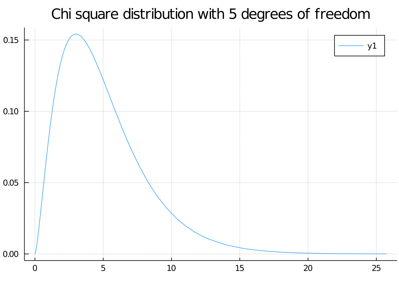
It turns out that this sample statistic approximately follows a Chi squared distribution with 4 - 1 = 3 degrees of freedom.

Why subtract 1?

Hypothesis tests and P values quantify the implausibility of the null hypothesis.

Let’s be optimistic, and assume that we generated data correctly from the uniform distribution.

123 GO: What’s our null hypothesis?

using Distributions
import HypothesisTests

# P-value calculation
chi_rv = Chisq(length(counts) - 1)
pval1 = 1 - cdf(chi_rv, chi_stat)
0.753004311656458

# Verify statistic and pvalue calculation with external library
test_one = HypothesisTests.ChisqTest(counts)

Pearson's Chi-square Test
-------------------------
Population details:
    parameter of interest:   Multinomial Probabilities
    value under h_0:         [0.25, 0.25, 0.25, 0.25]
    point estimate:          [0.35, 0.25, 0.2, 0.2]
    95% confidence interval: [(0.15, 0.5788), (0.05, 0.4788), (0.0, 0.4288), (0.0, 0.4288)]

Test summary:
    outcome with 95% confidence: fail to reject h_0
    one-sided p-value:           0.7530

Details:
    Sample size:        20
    statistic:          1.1999999999999997
    degrees of freedom: 3
    residuals:          [0.894427, 0.0, -0.447214, -0.447214]
    std. residuals:     [1.0328, 0.0, -0.516398, -0.516398]

Visualization and formal statistics complement each other.

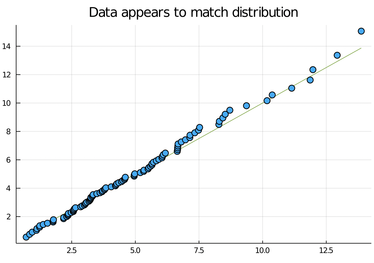
Summarizing: We’ve seen three methods to check whether data is different from a reference distribution:

1. Histograms
2. QQ plots
3. Chi square test

These techniques apply to data generated from any distribution, which make them powerful tools for checking parametric assumptions.

Exercise

See Canvas quiz